Process Altum images with Metashape

To process a project with Agisoft Metashape please follow the step-by-step instructions. You may download a dataset from this link.

General recommendations

• WingtraOne datasets, in particular captured with the Micasense Altum sensor, can be very large. Please make sure to have enough computing resources available.
• We recommend >= 32GB RAM, >6 core and enough high-speed SSD storage. 

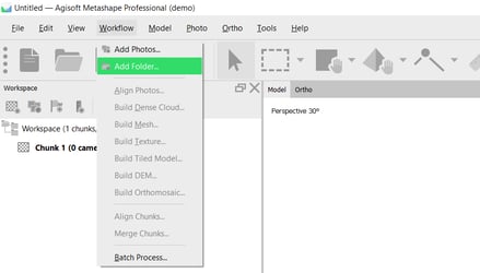
Step 1— Open Metashape and create project

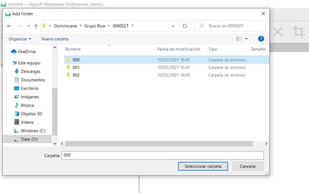
You can add pictures manually from a folder or select the complete folder. If you have more than one folder, you can select one folder and then add more folders.

Make sure to include the images of the calibration panel.

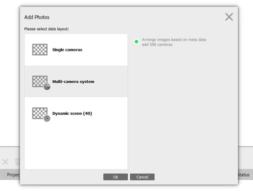
Step 2— Select Multi-camera system

When processing multispectral data sets, it's important to select multi-camera system in order to process correctly

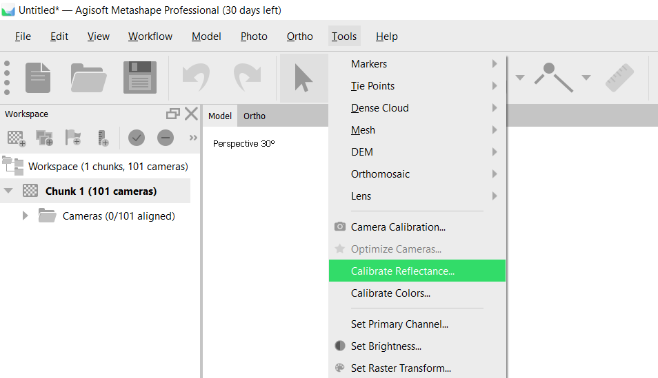
Step 3— Calibrate camera

In order to compare the information to other measuring tools, to satellite imagery, or even to compare through time, it is important that the images are calibrated radiometrically.

See this article to understand how to use the calibration panel.

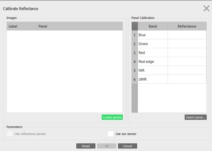
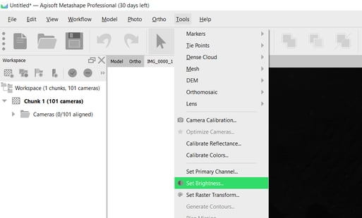
For this, select Tools and then Calibrate Reflectance...

Under Calibrate Reflectance, choose Locate Panels and the software will look for the pictures of the reflectance panel and show the reflectance numbers.

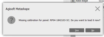
Note: a warning message showing there's a panel calibration missing will show up. This is because the thermal does not need the reflectance calibration.

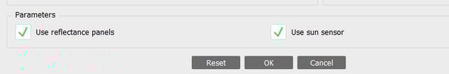
Note: before closing the reflectance calibration window, make sure to tick the Use reflectance panel and Use sun sensor boxes options.

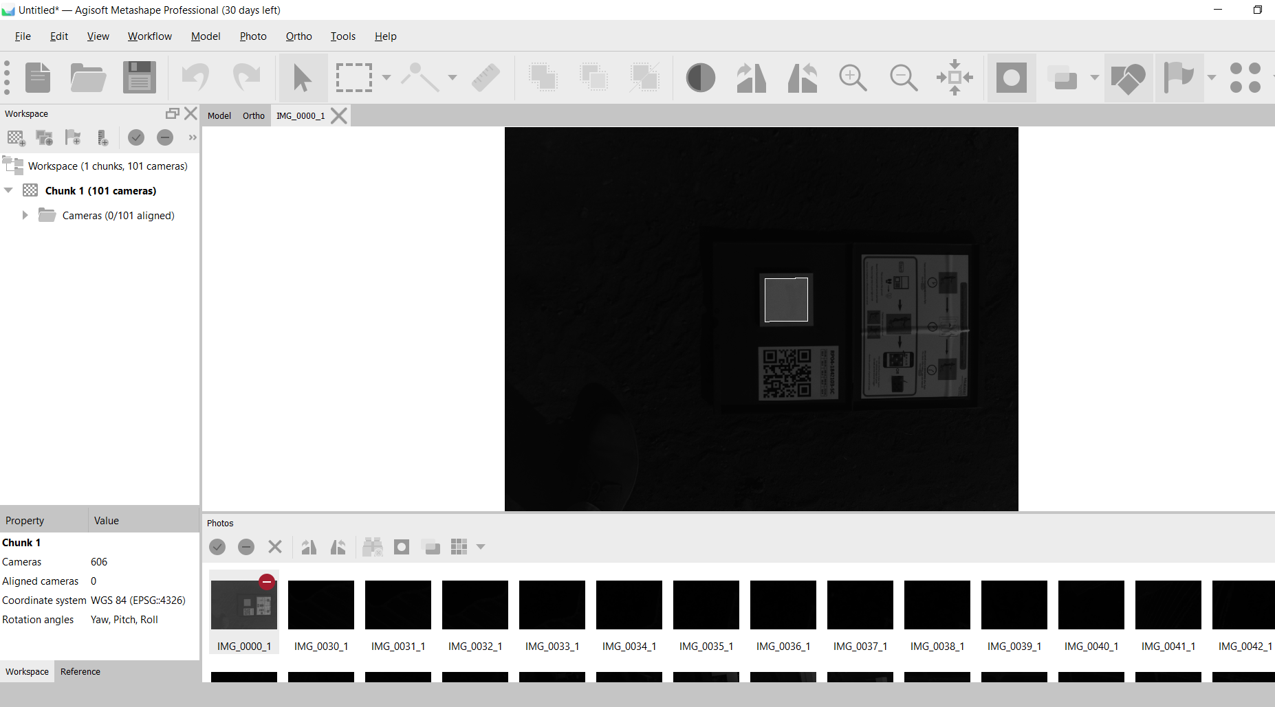
When checking the individual pictures, you should see that the software has chosen the grey square in the calibration panel.

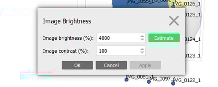
Set Brightness: Go to Tools and select Set Brightness...

Select Estimate and then Apply

Step 4— Align Photos

Go to Workflow and select Align Photos...

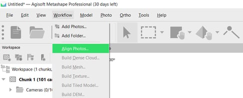
We recommend using High Accuracy and that you tick the "Generic preselection" and "Reference preselection" boxes

Step 5— Build Dense Cloud

Go to Workflow and select Build Dense Cloud...

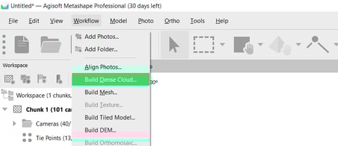
We recommend using High Quality for better results. Note that this can make the processing take longer.

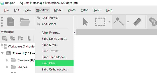
Step 6— Build DEM

Go to Workflow and select Build DEM...

We recommend using High Quality for better results. Note that this can make the processing take longer.

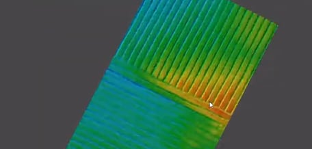
The DEM is the Digital Elevation Model which can give you precise information on the Surface model and where the water will flow to. Note that in Agriculture you might be able to see lines in the terrain.

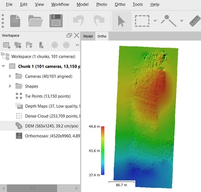
You can view the DEM by double-clicking on DEM under Chunk1 and see the map with different colors showing the heights.

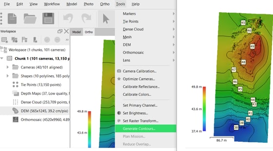
You can even see the Countour Lines by clicking on Tools and Generate Contours...
Here you can choose the invertal measured in meters and set the min and max altitude

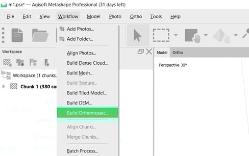
Step 7— Build Orthomosaics

Go to Workflow and select Build Orthomosaic...

Note that the software will take some time since it needs to create 6 orthomosaics (one for each band)

You can view the Orthomosaic by double-clicking on Orthomosaics under Chunk1 

Step 8— Generate Indexes

Go to Tools and select Set Raster Transform...

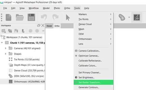
This will open a calculator where you can create your own formulas

You can write whichever formula you are interested in and go to the Palette tab to chose the combination of colors you want. After choosing the band and colors, select the Range (or click on Auto) and then click on Apply. You will see how the map changes colors in the back.

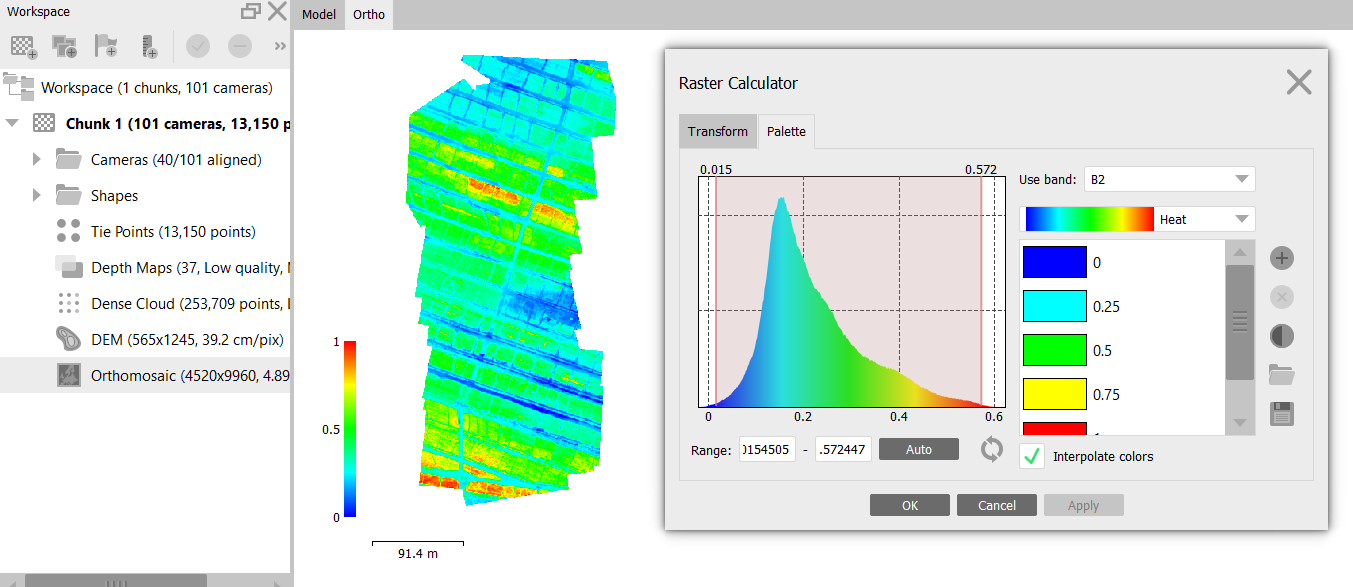
Basic formulas are:

• NDVI = (NIR-RED)/(NIR+RED) = (B5-B3)/(B5+B3)
• NDRE = (NIR-Red Edge)/(NIR+Red Edge) = (B5-B4)/(B5+B4)
• Thermal = LWIR = (B6/100) - 275.1

Note that in order to visualize, the thermal map needs the special formula mentioned above to get the values in Cº

If you'd like to see more examples and understand more about exporting the data, please check Metashape's Knowledge Base.